Uprights and Hub Assemblies: Penn Electric Racing REV12
REV12 is Penn Electric Racing's four-wheel-drive electric Formula SAE car, with a motor and planetary gearbox packaged inside every wheel. I own the design of its uprights and hub assemblies: the parts that carry every tire, braking, and drive load from the wheel into the suspension.
I built the load cases from first principles in MATLAB, checked them against the team's legacy spreadsheet, and validated the design with a nonlinear multibody FEA of the full bolted assembly in ANSYS. The final upright holds a 2.3x minimum safety factor across the worst-case load cases at 17% less mass than the starting design. It is machined from 7075-T6 aluminum and assembled with 4340 steel NAS fasteners, designed in SolidWorks and analyzed in ANSYS Mechanical to NASA-STD-5020 and ASME Y14.5.
The Problem
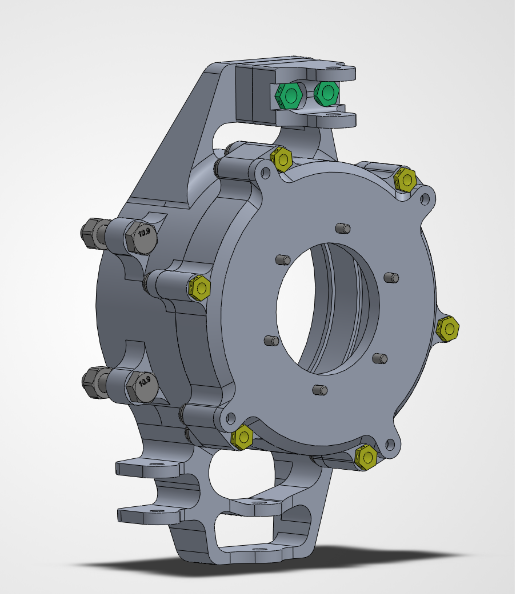
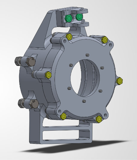
With a hub motor, the upright stops being a simple bracket between two ball joints. REV12's gearbox is a carrier output planetary: the ring gear is held stationary in the upright and the planet carrier drives the wheel. That means the upright has to package the motor, hold the ring gear, carry the wheel bearings and brake caliper, and react the full gearbox torque, all inside a 10 inch wheel.
On top of the usual tire and braking loads, the upright reacts the drive torque coming back through the ring gear and the motor's own inertia cantilevered off its mounts at 2.4 g lateral and 1.75 g braking. The hardest tradeoff was axial space. Spreading the wheel bearings apart lowers their loads, but every millimeter of bearing spread is a millimeter the motor and gearbox can't use.
I also designed a ring gear output version of the gearbox, where the ring gear drives the wheel instead of the carrier, which cut axial length 55%. It wasn't adopted for this season, but it's a candidate for future cars.
Starting From the Loads: Hand Calcs in MATLAB
Before touching geometry I needed loads I could trust, so I rebuilt the team's wheel hub load spreadsheet as a parameterized MATLAB model. Each load case starts at the vehicle level with longitudinal and lateral load transfer and aero downforce, giving a normal, lateral, and longitudinal force at every tire. Every combined case is checked against the friction circle, so no case asks a tire for more grip than it can produce.
From there I wrote full 3D force and moment equilibrium on the hub. The Matlab script outputs the bearing loads that the wheel hub applies on the uprights.
Wheel Hub Load Hand Calcs
%params
m = 300;
g = 9.81;
Wf = 0.45;
hcg = 0.278;
Dwb = 1.530;
Dtf = 1.177;
Dtr = 1.162;
glat = 2.4;
gacc = 1.49;
gbrake = 2.16;
faero = 2716/4;
mu = 1.3;

brakeBias = 0.598180;
accBias = 0.6;

%calipers
fcaliperfront = [0;-1592.46;0];
fcaliperrear = 0;

rtire = 0.203;
rrotor = 0.18923;

d2 = 0.031624;
d3 = 0.01465;
d4 = 0.056;

%front
%load transfer front
dfLong = (m*g*gbrake*hcg)/(2*Dwb);
dfLat = (Wf*m*g*glat*hcg)/(Dtf);
dfNormal = m*g/2*Wf;
dfaero = faero;

%normal front
fnlonglat = [0;dfNormal+dfLong+dfLat+dfaero; 0];
fnlat = [0; dfNormal+dfLat; 0];

%lateral front
flatlonglat = [-mu*fnlonglat(2);0;0];
flatlat = [-mu*fnlat(2);0;0];

%longitudinal front
flonglonglat = [0;0;-m*g*gbrake*brakeBias/2];
flonglat = [0;0;0];

%rear
%load transfer rear
drLong = (m*g*gacc*hcg)/(2*Dwb);
drLat = ((1-Wf)*m*g*glat*hcg)/(Dtr);
drNormal = m*g/2*(1-Wf);

%normal rear
rnlonglat = [0;drNormal+drLong+drLat+dfaero;0];
rnlat = [0;drNormal+drLat;0];

%lateral rear
rlatlonglat = [-mu*rnlonglat(2);0;0];
rlatlat = [-mu*rnlat(2);0;0];

%longitudinal rear
rlonglonglat = [0;0;m*g*gacc*accBias/2];
rlonglat = [0;0;0];

syms b1y b2y b1z b2z b1x b2x real

b1 = [b1x;b1y;b1z];
b2 = [0;b2y;b2z];

%solve
lcase = [2,2]; %1 is front 2 is rear for the first value, 1 is longlat 2 is lat for the second value

if lcase(1)==1
    if lcase(2)==1
        eqlong = flonglonglat;
        eqlat = flatlonglat;
        eqnormal = fnlonglat;
        eqcaliper = fcaliperfront;
    else
        eqlong = flonglat;
        eqlat = flatlat;
        eqnormal = fnlat;
        eqcaliper = [0;0;0];
    end
else
    if lcase(2)==1
        eqlong = rlonglonglat;
        eqlat = rlatlonglat;
        eqnormal = rnlonglat;
        eqcaliper = [0;0;0];
    else
        eqlong = rlonglat;
        eqlat = rlatlat;
        eqnormal = rnlat;
        eqcaliper = [0;0;0];
    end
end

eqlongdis = [-d2-d3;0;0];
eqlatdis = [-d2-d3;-rtire;0];
eqnormaldis = [-d2-d3;0;0];
eqb2dis = [d4;0;0];
eqcaliperdis = [-d3;0;0];

% Solve force-balance equations for the front contact forces
fnet = b1 + b2 + eqlong + eqlat + eqnormal + eqcaliper == 0;
mnet = cross(eqlongdis,eqlong)+cross(eqlatdis,eqlat)+cross(eqnormaldis,eqnormal)+cross(eqb2dis,b2)+cross(eqcaliperdis,eqcaliper)==0;
solution = solve([fnet; mnet], [b1x, b1y, b1z, b2y, b2z]);

b1val = double(subs(b1, solution));
b2val = double(subs(b2, solution));

T = array2table([b1val' b2val'], ...
    'VariableNames', {'B1x','B1y','B1z','B2x','B2y','B2z'});
disp('Bearing Loads [N]')
disp(T)
Writing the problem out this way exposed errors the spreadsheet had carried for seasons. Its combined load case added two totals that each already contained the static weight, inflating combined loads by about 37 to 39%. It left out the axial bearing force from cornering entirely, stacked peak braking and peak cornering past the friction circle. It also ran a 2.4 g cornering case with no aero downforce, which is beyond the car's roughly 2.09 g rollover limit, so aero had to be included for that case to be physical.
The script produces two sets of bearing loads for the front and the rear. Max lateral and max longituinal and just max lateral.
I also wrote a second script solves for the forces in the upper and lower control arms, tie rod, and pushrod from the suspension hardpoint coordinates, including spring deflection under load. I validated it with equilibrium closure checks and an independent cross product check, which caught a sign error from mirroring between the vehicle and CAD coordinate frames. The script is basically a 6 DOF load solver for the two force members in the suspension system. The solver first calculate spring compression from the tire vertical load and then it finds the suspensino linkage positions. Then the solver treats the entire system as a statics problem and solve for the forces in each linkage given the lateral, longitudinal and normal load cases.
Multibody FEA of the Upright Assembly
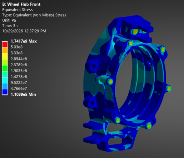
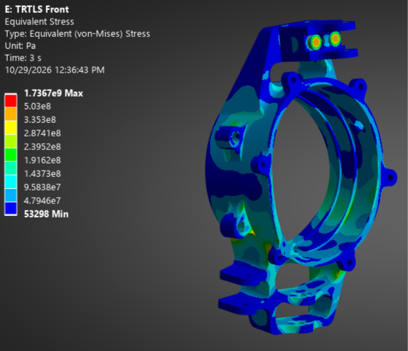
I modeled the upright as the real assembly of separate bodies rather than one bonded solid. A bonded model behaves like a single machined part, so it can't show what actually fails a bolted assembly: joints gapping open, interfaces slipping, or load taking an unexpected path between parts. The upright, bearing plates, camber bracket, shim, and every NAS fastener are separate bodies joined by frictional contact.
The 7075-T6 parts use a bilinear isotropic hardening model so local yielding at stress concentrations is captured instead of reported as an unrealistically high elastic peak, and they are judged by von Mises stress. Compressive regions such as the bearing seats are judged by minimum principal stress. The model is linked to SolidWorks through the associative reader, and named selections are built from rule-based criteria rather than hand-picked faces, so contacts and loads stay attached every time the CAD changes.
Fixing the Boundary Conditions
My first setup fixed the remote displacements at each control arm hardpoint in all six degrees of freedom. That told ANSYS the upright was welded rigidly to the suspension at every pickup, so the supports could react bending moments that a spherical joint physically can't carry. The result looked stiffer than the real part, and stress gathered around the upper control arm bracket instead of following the true load path through the upright.
I changed each hardpoint to fix the three translations and leave all three rotations free, which is how a ball joint actually behaves. With the supports only able to push and pull, the loads coming in through the bearing seats had to travel through the upright body to reach the control arms, and the hardpoint reactions could be checked directly against my MATLAB link force solver. Comparing reaction forces to the hand calcs became a standard step after every solve.
I also conducted a second Ansys static structural study where I fixed the wheel hub at the bearing and applied control arm loads to upper control arm and lower control arm connectino points. From the matlab calculations the forces were actually very similar to the force reactions from the ansys study where I fixed the control arm/tie rod points. However, in this study I had the forces going straight into and out of the control arm points laterally to be conservative which is why it sees more stress.
Both ansys simulations had 3 different steps, the first one for preloading the bolted joints, the second one for max lateral and max longitudinal load case, and the third one for the max lateral load case.
Modeling Bolted Joints in ANSYS
The bolted joints were the hardest part of the model to get right, and the place where a plausible-looking setup most easily gives the wrong answer. I sized preload for the NAS6203 (#10-32) and NAS6204 (1/4-28) fasteners per NASA-STD-5020, carrying both a maximum preload (25% tightening scatter) to check bolt and thread strength and a minimum preload (scatter plus 5% embedment relaxation) to check joint separation and slip. Every thread in the aluminum runs into a screw-lock Heli-Coil insert, so its prevailing torque is added on top of the installation torque.
The solve runs in three load steps. In the first, each bolt is pulled to its preload. In the second, the bolt's tightened length is locked so it behaves like a real torqued fastener. In the third, the bolts stay locked while the external loads ramp on from zero, so the joint only sees service loads after it is clamped. One trap I hit early: leaving the later steps set to apply a preload of zero doesn't hold the clamp. It models a bolt that was never tightened.
The contact setup mattered just as much. ANSYS's automatic contact detection bonded each bolt shank to the wall of its hole, which short-circuits the load path and reports almost no clamp pressure even with full preload applied, so I suppressed those contacts. The clamped faces use Augmented Lagrange contact with small gaps closed at the start, so CAD tolerances don't read as an open joint. My pass criterion was a closed, sticking ring of contact around every bolt that survives the full external load without turning to sliding or gapping.
ANSYS isn't built to check bolt shear, so I ran bolt margins as hand calcs to NASA-STD-5020 alongside the FEA. Grip lengths are chosen so the unthreaded shank, not the threads, sits in every shear plane, and close-fit holes are match-reamed through the stack.
Ring Gear Shrink Fit
In a carrier output gearbox the ring gear never turns, so the joint between the ring gear and the upright has to react the full gearbox torque. I compared a keyed fit against an interference fit for torque capacity, then settled on an m7 shrink fit. The aluminum upright is heated so its bore grows, the steel ring gear drops in, and the joint locks as the upright cools.
I sized the fit with the Lamé thick-walled cylinder equations for the 7075-T6 upright and the nitrided 4140 ring gear. Interference sets the contact pressure between the two parts, and that pressure, through friction across the contact area, sets the torque the joint can carry before it slips. The fit has to work at both ends of its tolerance band: at minimum interference it still has to hold peak drive torque with margin, and at maximum interference the hoop stress in the aluminum has to stay below yield.
Temperature makes the minimum case harder. Aluminum expands roughly twice as fast as steel, so as the hub heats up on track the bore grows away from the ring gear and the fit loosens. I checked the minimum interference at operating temperature, not just at room temperature, and controlled total runout on the bore so the ring gear stays concentric with the wheel bearings.
Letting the Loads Drive the Geometry
Once the loads and the model were right, the geometry had to follow. Correcting the legacy load cases cut the inflated combined loads by more than a third, but also added the cornering axial bearing load that had never been counted. That meant removing material where the old numbers had overbuilt the upright and reinforcing the regions that carry axial load.
With the corrected boundary conditions in place, the von Mises results showed which regions were doing real work under every load case and which were along for the ride. I removed material from the low-stress regions and checked each iteration against the full load set, which brought the upright down 17% in mass while holding a 2.3x minimum safety factor.
The bearing spacing came straight from gearbox requirements. The control arm spacing came straight from suspension hardpoints. Packaging also forced a change to the sealing, since there was only about 0.125 in of radial land on each side of the bearing bore, too narrow for a standard face seal groove, so the seal was resized to a 2 mm cross-section O-ring in a groove toleranced to ISO 3601-1.
Results
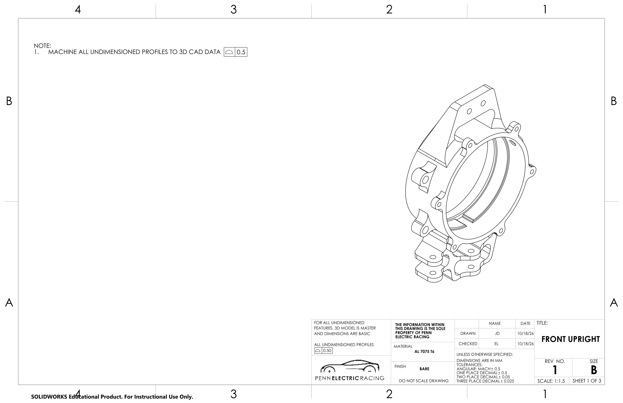
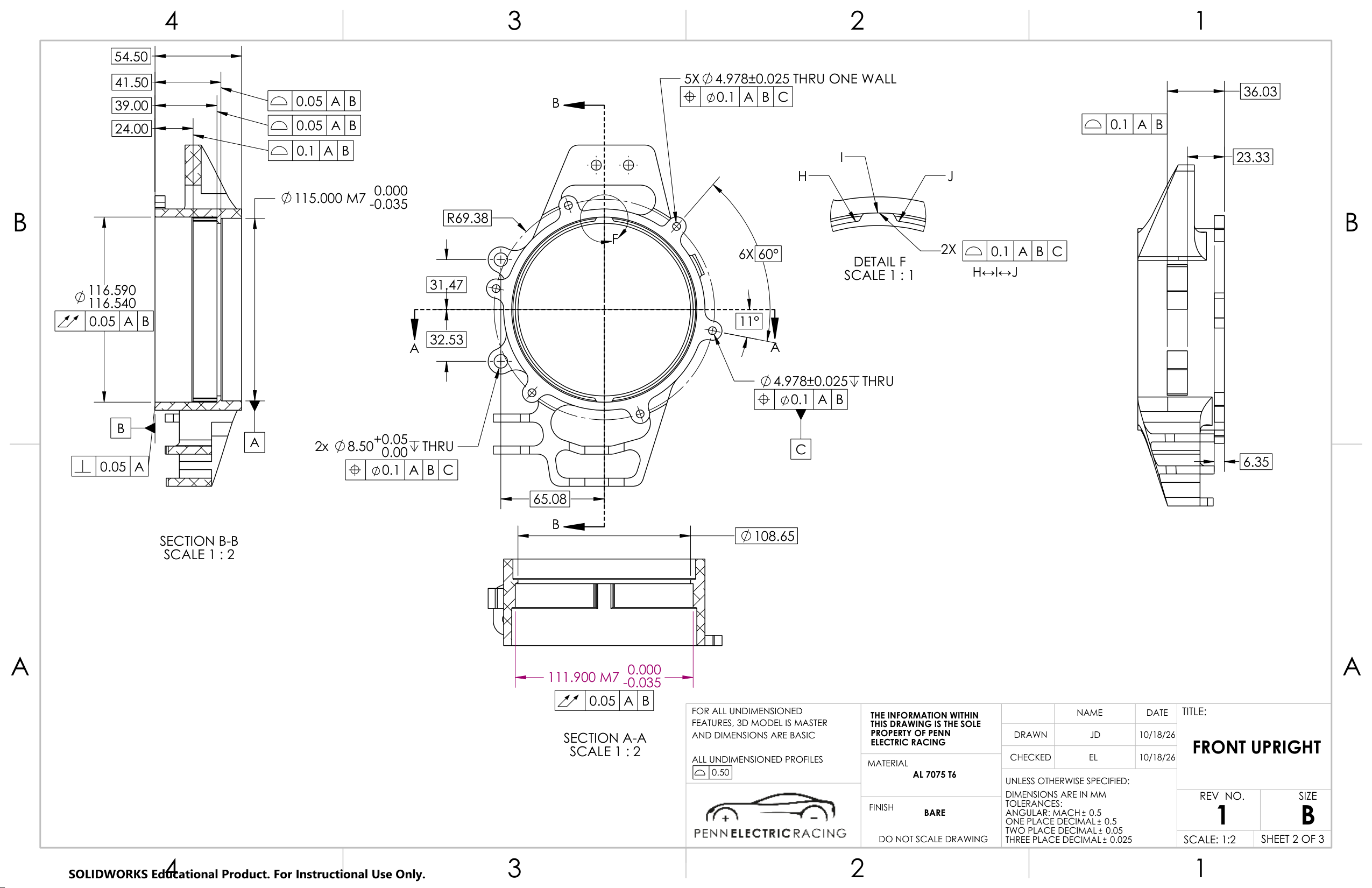
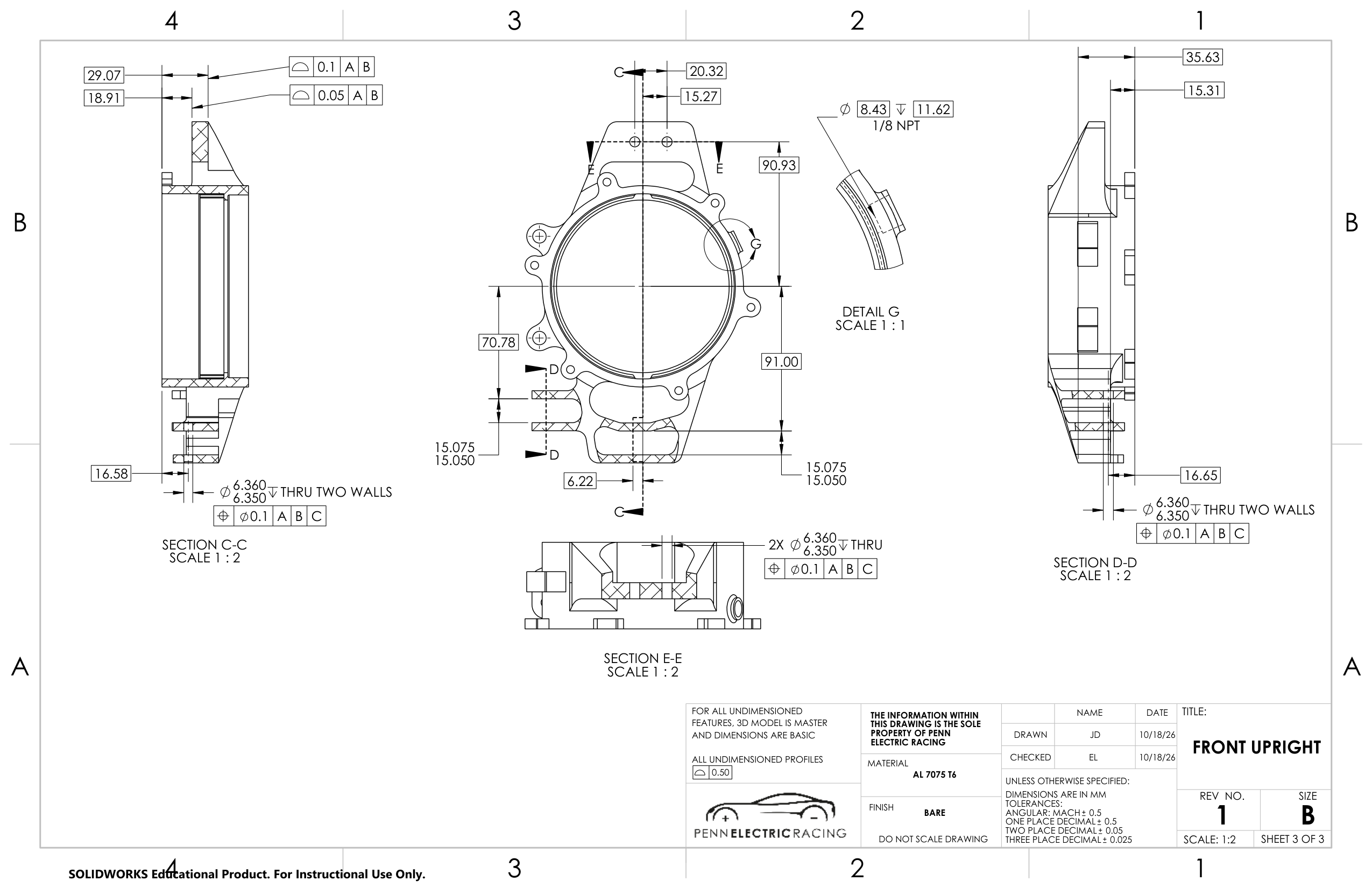
The final upright holds a 2.3x minimum safety factor across every worst-case load case at 17% less mass. I released its GD&T drawings to ASME Y14.5 to external CNC manufacturers, with the tolerance stack-up checked across the upright and gearbox interface.
What I Learned
- Audit inherited calculations before trusting them. The legacy spreadsheet had been reused for seasons, and its biggest error overstated combined loads by more than a third while missing a load entirely. Rewriting it symbolically made every assumption visible.
- Boundary conditions and contact setup matter more than mesh density. Fully fixed hardpoints, one auto-generated bonded contact, or one pretension step set wrong all produce clean, convincing, and wrong results. Checking reaction forces and contact status against hand calcs became part of every solve.
- Know where the solver stops being the right tool. Bolt shear, preload scatter, and fit tolerances are faster and more defensible as hand calcs to a standard than as FEA output, so the two methods ran side by side throughout the project.